Page contents :
    Create benchmark datasets
    Table 1 (motif properties)
    Running MotifSuite on the benchmark datasets
    Computation of performance indicators
    Table 2 (MotifSampler performances)
    Table 3 (MotifRanking performances)
    Table 4 (FuzzyClustering performances)

References

Gama-Castro, S. et al. (2008) RegulonDB (version 6.0): gene regulation model of Escherichia coli K-12 beyond transcription, active (experimental) annotated promoters and Textpresso navigation, Nucleic Acids Research, Vol. 36, Database issue:D120-4.

Create benchmark datasets

The benchmark datasets consisting of 43 E.coli sequence datasets each containing a known motif derived from RegulonDB are created as follows: RegulonDB is a database on transcription regulation and operon organization in Escherichia coli. We start with the file 'TF Binding Sites' (http://regulondb.ccg.unam.mx/download/Data_Sets.jsp). For each of 43 distinct transcription factors, we select the first target gene of each transcription unit regulated by this transcription factor, and for each target gene, we select the intergenic region 250 nucleotides upstream and 50 nucleotides downstream of the translation start site (as the transcription start site is often unknown). This gives for each transcription factor a file in FASTA format with a list of DNA sequences (separated by '>') for each target gene.
Based on the genome coordinates for all transcription factor binding sites described in 'TF Binding Sites', we describe the motif model that corresponds to the transcription factor in each dataset by the relative start and end position, strand and nucleotide description of the sites in the created sequences dataset. Secondly, we use the positional nucleotide counts from the file 'Matrices_Alignments' to create a PWM representation of the motif model.
(download Datasets).

Table 1 (motif properties)

The benchmark datasets consist of 43 distinct FASTA files each describing a set of DNA sequences. The known motif hidden in each of these files is described by a PWM and by a set of annotated instances for each of 43 distinct transcription factors.

Table 1 lists motif and dataset properties for the different transcription factors.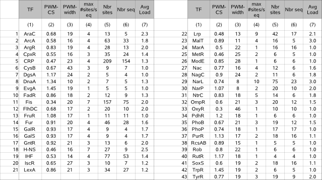

The motif properties in our benchmark lay within the following ranges (exceptions between brackets) :
Column (1) : TF = Transcription Factor identifier, alphabetically listed from 1 to 43
Column (2) : PWM-CS = motif consensus score computed from the PWM representation of regDB, between 0.45 and 1.45 (0.30, 0.34)
Column (3) : PWM-width = motif width (fixed for all instances), between 7 and 27 (37,42)
Column (4) : max #sites/seq = maximum number of instances in a sequence of the fasta file, between 1 and 4 (5,7,9,10)
Column (5) : Nbr sites = total number of instances over all sequences in the fasta file
Column (6) : Nbr seq = number of sequences in the fasta file, between 4 and 33 sequences (53,75,154).
Column (7) : Avg Load = indicator for the average (avg) number of instances (load) per sequence, computed as ['Nbr sites' minus 'max #sites/seq'] divided by ['Nbr seq' - 1 ], assuming that one sequence has the maximal number of instances known to be present in the dataset(4) and all other sequences have the same number of instances.

Case study: running MotifSuite on the benchmark datasets

The main goal of this case study is to evaluate the motif detection performance of MotifSamplers new release (3.1.5) and to study the pros and contras of the two different prioritizing tools MotifRanking and FuzzyClustering. The results of the case study are discussed in the respective guidelines of each application. This section describes how the applications have been run on the benchmark datasets (input, parameter settings and selection of the output). The workflow presented in the next figure is applied on each dataset and the whole procedure is repeated 10 times to average out particularly good or bad results that may be obtained by chance in the stochastic framework of MotifSampler.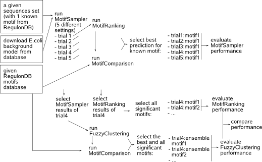

We run MotifSampler in a predefined set of trials that mainly differ in the setting for parameter -p (5 trials as described in table 2a). For each trial, we run MotifRanking with default program parameter settings on the PWM output file reported by MotifSampler to extract different motifs in sorted motif score order and we compare the respective motif models to biologically true motif models in RegulonDB (database available on our server) using MotifComparison. From the list of reported motif models by MotifRanking in each trial, we retain the one with the highest LL score that was detected at least 10 times as the best motif prediction for the known motif in this trial. If no motif with a count higher than 10 was detected in a dataset, we retain the motif model with the yet highest motif count. At this stage, we can evaluate how well MotifSampler finds the known motif and the improvements (e.g. does it find the motif more frequently, is the total number of known instances better described) that can be achieved with the extended design (parameter -p and sampling technique) added in the current release 3.1.5 of MotifSampler. In what follows we further work with the results of MotifSampler obtained in 3.1.5-uniform trial unless MotifSamplers convergence rate was lower than 70, then we choose the results obtained in 3.1.5-fixed trial.
From the list of motifs reported by MotifRanking in the selected trial (3.1.5-uniform or 3.1.5-fixed trial), we also retain the motif that has a lower motif score than the first retained motif provided it has a motif count higher than 10. We re-evaluate redundancy between the two retained motifs using MotifComparison with pBliC-metric. We can now evaluate how the metrics in MotifRanking serve to find the most likely true motif model amongst a list a multiple MotifSampler solutions (metrics : LL-score as indicator to select the best motif, RR as significance measure, CS score as measure for conservation of the detected motif).
Next, we run FuzzyClustering with default program parameter settings on the total set of instances that was reported by MotifSampler (obtained in 3.1.5-uniform or 3.1.5-fixed trial). For each reported ensemble motif, we compare the motif model (PWM) to biologically true models in RegulonDB (database available on our server) using MotifComparison. We retain the first reported and -if present- the next reported ensemble motif. We can now evaluate the performance of FuzzyClustering in accurately finding the known motif instances and discuss the pros and contras of FuzzyClustering compared to MotifRanking.


Program commands :
MotifSampler : [-r 100, -s 0, -w as_known_from_RegulonDB -n 1 -x not_used -M as_known_from_RegulonDB -b Ecoli_order2].
3.1.5-default trial [-p 0.9_0.25, sampling technique(coded)], 3.1.5-higher trial [-p 0.9_0.75|b0.5, sampling technique(coded)], 3.1.5-fixed trial [-p f0_1|f0_0_1|f0_0_0_1], 3.1.5-uniform trial [-p u, sampling technique(coded)], 3.1.1[mimic]-uniform trial [-p u, averaging technique(coded)]
In what follows, w equals the motif width parameter -w used in MotifSampler.
MotifRanking : [-x = 0.5*w, -s = w, -t 0.4, -m 0, -r 5].
FuzzyClustering : [-p 0.1 -i 0.5 -c 0.8*CS_as_known_from_RegulonDB -j 0.1].
MotifComparison : KL_metric:[-l = 0, -x = 0.5*w, -s = w, -t = 0.4] and p-BLiC_metric:[-l = 1, -x = 0.5*w, -s = w, -t = 0.001, -n = w, -p = program_default, -b = Ecoli_order2].

Computation of performance indicators

The following performance indicators are used throughout this study. Mark that for every performance indicator where the stochastic properties of MotifSampler may influence the result, the reported indicator is averaged over the result in 10 repetitions where MotifSampler was repeated on the same dataset with the same parameter settings.

- Conv = convergence rate of MotifSampler = the number of solutions (PWMs) reported by MotifSampler. Ideally this number equals the number of runs as set by parameter -r in MotifSampler. The convergence rate will be lower if MotifSampler does not report a solution for all runs. Run abortion happens when at some point in a run too few instances are being allocated in the total sequence dataset.
- N = motif detection count = the number of solutions reported by MotifSampler that represent this same motif. The count N is computed by MotifRanking and reported as 'Total' in the text outputfile. N must be higher than at least 10 in order for any reported motif model to be considered as a statistically relevant solution.
- RR = return ratio of a motif = the fraction of MotifSampler solutions that report the same motif, RR = N/Conv. The higher RR, the higher the statistical significance of a solution and the more likely this solution represents a biologically true motif.

The PPV and sensitivity of a set of detected instances of a motif reflect how accurately this set describes the known (biologically true) instances in the dataset :
- PPV = measures the fraction of detected instances that are true (an instance is true if it has at least 50% overlap with a known instance described in RegulonDB);
- sens = measures the fraction of the known instances described in RegulonDB that is reported in the set of detected instances.
A biologically true motif is best detected when PPV equals the highest value (1.00, there are no untrue instances reported) and sensitivity equals the highest value (1.00, all true instances are detected). When motifs are more difficult to find, the program parameters in MotifSampler may be adapted to balance the motif search towards only true instances (high PPV, at the cost of missing our some true instances) or towards finding all true instances (high sens, at the cost of including some untrue instances).

Indicators specific for FuzzyClustering :
- Occ(i) = weighted average instances occurency (reported as weighted_average_occurency in #instance memberships) is computed as the sum of all instance occurencies (occ) each multiplied with their instance membership, normalized by the total sum of all instance memberships. An instance occurency (occ) is computed as the number of times this instance (or a shifted version) was present in the list of de-novo detected motifs by MotifSampler. Occ(i) is an indicator for the number of times (an instance of) an ensemble motif was (on average) detected by the multiple runs in MotifSampler.
- N(m) = weighted motif count (reported as weighted_count in #motif memberships) is computed as the sum of all motif memberships normalized by the highest motif membership reported for the ensemble motif. N(m) is an indicator for the number of de novo detected motifs by MotifSampler that support the retained motif (correspond to the same motif as the retained ensemble motif).

Table 2 (MotifSampler performance)

(back to : case study)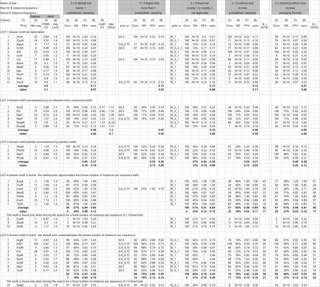
Table 2 - columns (5-8) list the performance indicators (Conv, RR, PPV, sens) computed for the best motif (*) detected for a given dataset by running MotifSampler in 5 predefined trials that each represent a different setting for the program parameter -p and/or a different way to derive the number of instances per sequence (probabilistic sampling or conservative averaging formula). Columns (2-4) display properties of the dataset and the known true motif, extracted from table 1. The 43 datasets are sorted into 5 different lists depending on how well a motif was detected by MotifSampler (list-1 : no motif detected, list-2 : unknown motif detected, list-3 : known motif instances partially detected, list-4 and -5 : known motif instances well detected, list-4 and list-5 differ in the average number of known true instances per sequence of the dataset)

Column (1) : TF = Transcription Factor identifier of a given dataset
Column (2) : Nbr seq = number of sequences in the dataset, extracted from table 1
Column (3) : PWM-CS = consensus score (representing the strength of overrepresentation) of the RegulonDB motif model, extracted from table 1
Column (4) : Avg Load = indicator for the average number of known instances per sequence in a dataset, extracted from table 1
Column (5) : Conv = convergence rate of MotifSampler = number of runs (out of 100 initiated runs) that report a solution
Column (6) : RR = return ratio of the detected motif = fraction of solutions that reports the same detected motif
Column (7) : PPV = positive predictive value of the detected motif = fraction of detected motif instances that are known to be true
Column (8) : sens = sensitivity of the detected motif = fraction of known instances that is reported by the detected set of motif instances
Column (9) : motif-CS = consensus score of the detected motif PWM

(*)(**)
(*) For each trial and each dataset, MotifSampler reports a list of multiple solutions. The best motif from this list is selected (by MotifRanking) as the motif model with the highest LL score that is statistically significant (count N>10). If none of the candidate motifs is statistically significant, the 'best' motif is defined as the one with the yet highest count N (the most statistically significant one).

Table 3 (MotifRanking performance)

Table 3 - columns (6-11) list the performance indicators (N, RR, PPV, sens, CS, LL) computed for the candidate true motif(s) (*) retained for a given dataset by running MotifSampler and MotifRanking on 43 benchmark datasets. Columns (2-4) display properties of the dataset and the known true motif, extracted from table 1. The 43 datasets are sorted into 2 lists depending if MotifRanking reported a significant motif (RR and/or N >10) or not.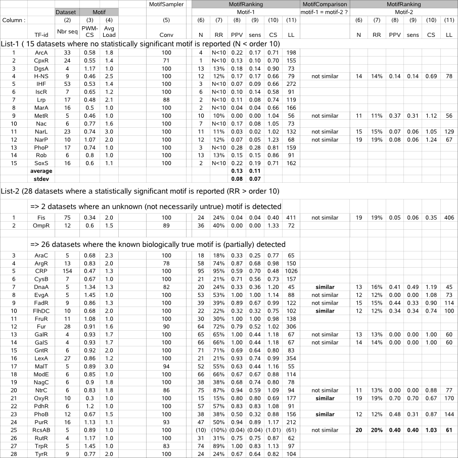

Column (1) : TF = Transcription Factor identifier of a given dataset
Column (2) : Nbr seq = number of sequences in the dataset, extracted from table 1
Column (3) : PWM-CS = consensus score (representing the strength of overrepresentation) of the known motif in the dataset, extracted from table 1
Column (4) : Avg Load = indicator for the average number of known instances per sequence in a dataset, extracted from table 1
Column (5) : Conv = convergence rate of MotifSampler = number of runs (out of 100 initiated runs) that report a solution
Column (6) : N = motif count = number of solutions that represent the same detected motif
Column (7) : RR = return ratio of the detected motif = fraction of solutions that reports the same detected motif (=N/Conv)
Column (8) : PPV = positive predictive value of the detected motif = fraction of detected motif instances that are known to be true
Column (9) : sens = sensitivity of the motif = fraction of known instances that is reported by the detected set of motif instances
Column (10) : CS = consensus score of the detected motif PWM
Column (11) : LL = LogLikelihood score of the detected motif as computed in MotifSampler

(*) For each dataset, MotifRanking reorganizes the MotifSampler solutions in a shorter list of non-redundant motifs. If none of the retained solutions has a motif count higher than 10, we retain as motif-1 the solution with the yet highest count. Else, we retain as motif-1 the solution with the highest LL-score that has a count higher than 10 and as motif-2 (if so present) a lower LL-scoring solution that still has a motif count higher than 10 as possible candidates to be a biologically true motif.

Table 4 (FuzzyClustering performance)

Table 4 - columns (3-8) list the performance indicators (Occ(i), N(m), dM(i), CS, PPV, sens) computed for the candidate true motif(s) (*) retained for a given dataset by running MotifSampler and FuzzyClustering on 43 benchmark datasets. Column (1) displays properties of the known true motif, extracted from table 1. The 43 datasets are sorted into 2 lists depending if FuzzyClustering retained a significant motif or not.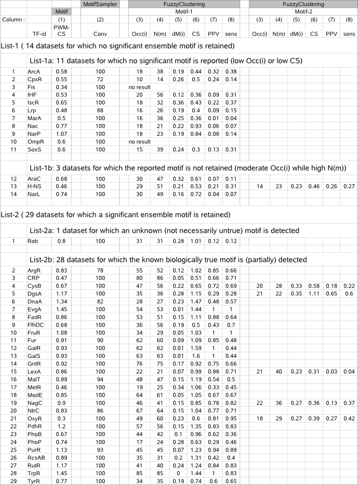

Column (1) : TF = Transcription Factor identifier of a given dataset
Column (2) : PWM-CS = consensus score (representing the strength of overrepresentation) of the known motif in the dataset, extracted from table 1
Column (3) : Conv = convergence rate of MotifSampler = number of runs (out of 100 initiated runs) that report a solution
Column (4) : Occ(i) = weighted average instances occurency = number of times an instance of the ensemble motif occurred on average in the supplied MotifSampler motifs (the contribution of each instance to this average is weighed by its instance membership in the ensemble motif)
Column (5) : N(m) = weighted motif count = number of MotifSampler motifs (the contribution is weighed with the motif membership in the ensemble motif) that correspond to the ensemble motif
Column (6) : dM(i) = the difference between the maximal and minimal instance membership score reported in the ensemble motif
Column (7) : CS = consensus score of the ensemble motif PWM
Column (8) : PPV = positive predictive value of the ensemble motif = fraction of ensemble instances that are known to be true
Column (9) : sens = sensitivity of the ensemble motif = fraction of known instances that is reported by the set of ensemble instances

(*) For each dataset, FuzzyClustering reorganizes the MotifSampler solutions in a shorter list of non-redundant ensemble motifs (subsets of instances that frequently occurred together in the MotifSampler solutions). If no ensemble motif was reported at default parameter settings, we report as motif-1 the ensemble motif obtained at less stringent settings (i.e. that allow for a less supported motif (lower N(m)) or a lower consensus score). Else, we retain as motif-1 and (if so present) motif-2 the solution(s) with the highest respectively second highest Occ(i) as possible candidates to be a biologically true motif.