MotifSampler's program parameter -p specifies Pr(x), the prior distribution on the number of instances of a motif in a sequence. The argument x equals the number of instances of a motif in a sequence and varies from zero to a maximal number set by the user (program parameter -M). Pr(x) is used in each iteration step of the motif detection process to calculate the number of instances of a motif that should be sampled in each sequence (read more in MotifSampler Guidelines, see fig.5).
!Mark that in case MotifSampler searches for multiple motifs in a dataset, the same prior Pr(x) is used for every repeated motif search.

Page contents :
Description of 5 types of prior distribution
Mathematical description
Graphical illustration

Description of 5 types for Pr(x)

We propose 5 models for a prior distribution Pr(x) :
Mark: operators < an > mark the definition of a variable, do not apply the operators in your entry for -p on the webinterface or commandline)

1) the default distribution,
assumes it will a priori always be more likely to find x copies than x+1 copies of a motif in a sequence.
Entry: -p <p_k>, with p = a value between 0 and 1 (0 and 1 excluded) and k = a value between 0 and 1 (1 excluded), p and k are separated by an underscore. The argument p describes the prior probability that a motif has exactly one instance in a sequence and k is a factor used to disfavor multiple instances of a motif in a sequence.
The default entry for -p is <0.9_0.25>. This prior will bias the motif detector towards sampling more or less 1 instance per sequence. With k=0.25, use p > 0.5 to have at least 50% chance of finding 1 instance in any sequence. An increasing k in the range [0.25->0.99] will slightly move the weight of the prior distribution towards multiple instances, but as k is defined to be smaller than 1, the peak of the prior distribution will always be on 1 instance per sequence. Using a value for p in the range [0.5->0.99] will minimize the probability of finding no instance in a sequence. See fig.1 for a visualization of some prior distributions at different combinations for p and k. As the computed probability for 3 instances per sequence is very low in all cases, it is recommended to set -M = 2 to avoid useless increase in runtime.

2) the uniform distribution,
Entry: -p u, assumes no a priori information at all. This distribution is by nature not limiting the number of instances so make sure -M is set to a reasonably limiting value.

3) the binomial distribution,
Entry: -p b<p>, with p same as defined in 1). This distribution needs to be used in combination with a reasonably limiting value for -M. The properties of this distribution are a mean = M*p and a variance = M*p*(1-p) on the number of instances per sequence. See fig.1 for a visualization of some prior distributions at different p.

4) the explicit distribution,
Entry: -p e<value0>_<value1>_... with <valueX> = a value between 0 and 1 (0 and 1 excluded) = the prior probability for X instances per sequence. E.g. e0.01_0.01_0.98 will bias the motif detector towards mainly 2 instances per sequence and -M is automatically set equal to 2 by the program.

5) the fixed distribution,
Entry: -p f<value0>_<value1>_... with <valueY> = a value between 0 and 1 (0 and 1 included) = probability for Y instances per sequence. This is however NOT a 'prior' probability distribution, but a posterior distribution that directly fixes the number of instances of a motif that will be sampled in each sequence of the dataset. E.g. f0_0_1 will search for exactly 2 instances in each sequence and -M is automatically set equal to 2 by the program.

Mathematical description

Here follows the mathematical description for each type of prior distribution :

C = normalization constant computed by the program,
M = maximum number of instances : internally computed value (i.e. Pr(x=M|Sk) < 0.001) or user parameter -M if this value is lower

1) default prior distribution = [(1-p)/C, p/C, k*p/C, (k^2)*p/C, (k^3)*p/C,..., (k^M)*p/C]
2) uniform prior distribution = [1/(M+1), 1/(M+1), 1/(M+1),..., 1/(M+1)]
3) binomial prior distribution = [(1-p)^M, M*p*(1-p)^(M-1),..., M!/(M-c)!/c! *p^c*(1-p)^(M-c),..., p^M]
4) explicit prior distribution = [Pr(0), Pr(1), Pr(2),..., Pr(M)]. The user supplied entries are normalized by the program.
5) fixed posterior distribution = [Pr(0), Pr(1), Pr(2),..., Pr(M)]. The user supplied entries are normalized by the program.

Graphical illustration

Ter illustration follows a graphical representation of some prior distributions at different parameter settings :

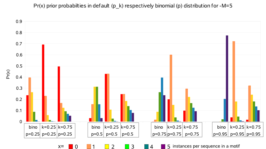
- Binomial distribution at M=5 for p=0.25, p=0.5, p=0.75, p=0.95 :
properties for p=0.25 : mean=1.25 and variance=0.94 ==> bias to 1 +/- 1 instance per sequence
properties for p=0.5 : mean=2.5 and variance=1.25 ==> bias to 2 to 3 instances per sequence
properties for p=0.75 : mean=3.75 and variance=0.94 ==> bias to 4 +/- 1 instances per sequence
properties for p=0.95 : mean=4.75 and variance=0.24 ==> bias to 5 instances per sequence

- Default distribution at M=5 for p=0.25, p=0.5, p=0.75, p=0.95 and k=0.25, k=0.75 :
properties for p=0.25 : ==> bias towards 0 instances per sequence
properties for p>=0.5 : ==> mainly bias towards 1 instance per sequence

Feedback

Contact us if you have comments, questions or suggestions or simply want to react on the contents of this guideline. Thank you.