Volume Visualization
 Run this m-file to see several examples of volume
 visualization in MATLAB(R).
 See also ISOSURFACE, STREAMTUBE, STREAMRIBBON,
          STREAMLINE, CONEPLOT.
Contents
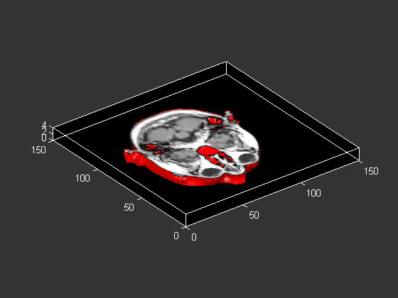
Isosurface of MRI Data
figure;
colordef(gcf,'black')
load mri;
D = squeeze(D);
[x y z D] = subvolume(D, [nan nan nan nan nan 4]);
p = patch(isosurface(x,y,z,D, 5), 'FaceColor', 'red', 'EdgeColor', 'none');
p2 = patch(isocaps(x,y,z,D, 5), 'FaceColor', 'interp', 'EdgeColor', 'none');
isonormals(x,y,z,D,p);
view(3);
daspect([1 1 .4])
colormap(gray(100))
camva(9);
box on
camlight(40, 40);
camlight(-20,-10);
lighting gouraud
Coneplot of Wind Data
figure;
colordef(gcf,'black')
cla
load wind
[cx cy cz] = meshgrid(linspace(71,134,10),linspace(18,59,10),3:4:15);
daspect([1 1 1])
h=coneplot(x,y,z,u,v,w,cx,cy,cz,y,3);
set(h,'EdgeColor', 'none');
colormap(hsv);
box on;
axis tight
camproj perspective;
camva(35);
campos([175 10 85]);
camtarget([105 40 0])
camlight left;
lighting gouraud

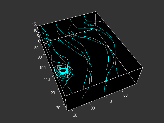
Streamlines of Wind Data
figure;
colordef(gcf,'black')
cla
[sx sy sz] = meshgrid(80, 20:10:50, 0:5:15);
h=streamline(x,y,z,u,v,w,sx,sy,sz);
set(h, 'Color', 'cyan');
daspect([1 1 1])
box on;
camproj perspective;
camva(32);
axis tight
campos([175 10 85]);
camtarget([105 40 0])
camlight left;
lighting gouraud
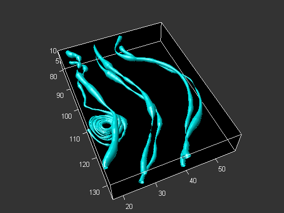
Streamtubes of Wind Data
Useful for visualizing divergence of a vector field
figure;
colordef(gcf,'black')
cla
[sx sy sz] = meshgrid(80, [20 30 40], [5 10]);
daspect([1,1,1]);
h=streamtube(x,y,z,u,v,w,sx,sy,sz);
set(h,'facecolor','cyan','edgecolor','none');
box on;
camproj perspective;
axis([70 138 17 60 2.5 16]);
axis tight
camva(28);
campos([175 10 95]);
camtarget([105 40 0])
camlight left;
lighting gouraud
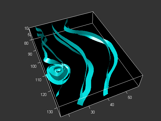
Streamribbons of Wind Data
Useful for visualizing curl of a vector field
figure;
colordef(gcf,'black')
cla
[sx sy sz] = meshgrid(80, [20 30 40], [5 10]);
daspect([1,1,1]);
h=streamribbon(x,y,z,u,v,w,sx,sy,sz);
set(h,'facecolor','cyan','edgecolor','none')
box on;
camproj perspective;
axis([70 138 17 60 2.5 16]);
axis tight
camva(28);
campos([175 10 85]);
camtarget([105 40 0])
camlight left;
lighting gouraud
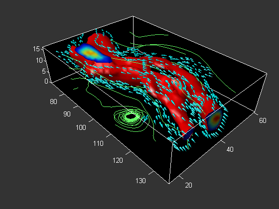
Isosurface, Isocaps, Coneplot, and Streamlines of Wind Data
figure;
colordef(gcf,'black')
cla
spd = sqrt(u.*u + v.*v + w.*w);
p = patch(isosurface(x,y,z,spd, 40));
isonormals(x,y,z,spd, p)
set(p, 'FaceColor', 'red', 'EdgeColor', 'none');
p2 = patch(isocaps(x,y,z,spd, 40));
set(p2, 'FaceColor', 'interp', 'EdgeColor', 'none')
daspect([1 1 1]);
[f verts] = reducepatch(isosurface(x,y,z,spd, 30), .2);
h=coneplot(x,y,z,u,v,w,verts(:,1),verts(:,2),verts(:,3),2);
set(h, 'FaceColor', 'cyan', 'EdgeColor', 'none');
[sx sy sz] = meshgrid(80, 20:10:50, 0:5:15);
h2=streamline(x,y,z,u,v,w,sx,sy,sz);
set(h2, 'Color', [.4 1 .4]);
colormap(jet)
box on
axis tight
camproj perspective;
camva(34);
campos([165 -20 65]);
camtarget([100 40 -5])
camlight left;
lighting gouraud