Tessellation and Interpolation of Scattered Data

This demo describes convex hulls, Delaunay tessellations, and Voronoi diagrams in 3 dimensions. It also shows how to interpolate three-dimensional scattered data.

Many applications in science, engineering, statistics, and mathematics use structures like convex hulls, Delaunay tessellations and Voronoi diagrams for analyzing data. MATLAB® enables you to geometrically analyze data sets in any dimension.

Here, in 3 dimensions, we show a set of 50 points with its convex hull.

% Create the data.
n = 50;
X = randn(n,3);
% Plot the points.
plot3(X(:,1),X(:,2),X(:,3),'ko','markerfacecolor','k');
% Compute the convex hull.
C = convhulln(X);
% Plot the convex hull.
hold on
for i = 1:size(C,1)
   j = C(i,[1 2 3 1]);
   patch(X(j,1),X(j,2),X(j,3),rand,'FaceAlpha',0.6);
end
% Modify the view.
view(3), axis equal off tight vis3d; camzoom(1.2)
colormap(spring)
rotate3d on

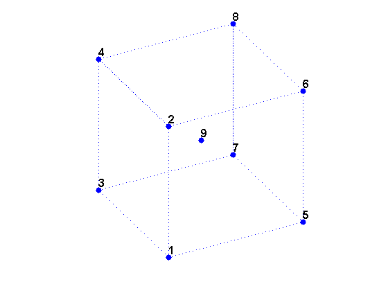
We can create a data set X of the 8 vertices of a cube plus its center.

X is a 9-by-3 matrix where each row is the 3-D coordinates of one point.

% Create X.
X = zeros(8,3);
X([5:8,11,12,15,16,18,20,22,24]) = 1; % Corners.
X(9,:) = [0.5 0.5 0.5]; % Center.
% Visualize X.
cla reset; hold on
d = [1 2 4 3 1 5 6 8 7 5 6 2 4 8 7 3];
plot3(X(d,1),X(d,2),X(d,3),'b:');
plot3(X(:,1),X(:,2),X(:,3),'b.','markersize',20);
t = text(X(:,1),X(:,2),X(:,3), num2str((1:9)'));
set(t,'VerticalAlignment','bottom','FontWeight','bold', 'FontSize',12);
view(3); axis equal tight off vis3d; camorbit(10,0);
rotate3d on

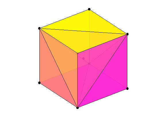
The convex hull of a data set is the smallest convex region that contains the data set. The convex hull of the cube data set X can be computed by CONVHULLN.

For this data set X, the convex hull has 12 facets, each corresponding to a row in K and plotted above with X. The cube is transparent so that you can see all the facets and data points.

% Compute the convex hull.
tri = convhulln(X);
% Plot the data
cla reset;
plot3(X(:,1),X(:,2),X(:,3),'ko','markerfacecolor','k');
% Plot the convex hull.
for i = 1:size(tri,1)
  c = tri(i,[1 2 3 1]);
  patch(X(c,1),X(c,2),X(c,3),i,'FaceAlpha', 0.9);
end
% Modify the view.
view(3); axis equal tight off vis3d
rotate3d on

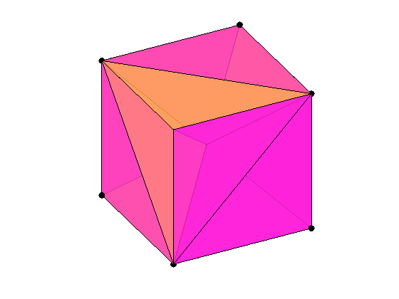
A Delaunay tessellation in 3 dimensions is a set of tetrahedrons such that no data points are contained in any tetrahedron's circumsphere. The Delaunay tessellation of the data set X can be computed by DELAUNAYN.

The 12 rows of T represent the 12 tetrahedrons that partition the data set X.

% Compute the delaunay tessellation.
tri = delaunayn(X);
% Plot the data.
plot3(X(:,1),X(:,2),X(:,3),'ko','markerfacecolor','k');
% Plot the tessellation.
for i = 1:size(tri,1)
  y = tri(i,[1 1 1 2; 2 2 3 3; 3 4 4 4]);
  x1 = reshape(X(y,1),3,4);
  x2 = reshape(X(y,2),3,4);
  x3 = reshape(X(y,3),3,4);
  patch(x1,x2,x3,(1:4)*i,'FaceAlpha',0.8);
end
% Modify the view.
view(3); axis equal tight off vis3d; camorbit(10,0)
rotate3d on

A Voronoi diagram partitions the data space into polyhedral regions, with one region for each data point. Anywhere within a region is closer to its data point than any other in the set. The Voronoi diagram of the cube data set X can be computed by VORONOIN.

V is the set of Voronoi vertices. C represents the set of Voronoi regions. For our data set X, C has 9 Voronoi regions. Here we show one Voronoi region, the region for the center point of the cube.

% Compute Voronoi diagram.
[c,v] = voronoin(X);
% Plot the data.
plot3(X(d,1),X(d,2),X(d,3),'b:.',X(9,1),X(9,2),X(9,3),'k.','markersize',20);
% Plot the Voronoi diagram.
nx = c(v{9},:);
tri = convhulln(nx);
for i = 1:size(tri,1)
   patch(nx(tri(i,:),1),nx(tri(i,:),2),nx(tri(i,:),3),rand,'FaceAlpha',0.8);
end
% Modify the view.
view(3); axis equal tight off vis3d; camzoom(1.5); camorbit(20,0)
rotate3d on

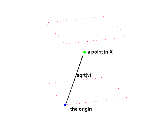
GRIDDATAN interpolates multidimensional scattered data. It uses DELAUNAYN to tessellate the data, and then interpolates based on the tessellation. We start with a data set of 500 random points in 3 dimensions and compute the values of a function, the squared distance from the origin, at each of these points.

% Create the data.
n = 500;
X = 2*rand(n,3)-1;
v = sum(X.^2,2);
% Draw a picture to show how X is defined.
cla reset; hold on
plot3([0.02, 0.47],[0.02,0.57],[0.02,0.57],'k-','linewidth',2);
plot3(0,0,0,'bo','markerfacecolor','b');
cube = zeros(8,3);
cube([5:8,11,12,15,16,18,20,22,24]) = 1; % Corners
cube(9,:) = [0.5 0.5 0.5]; % Center.
plot3(cube(d,1),cube(d,2),cube(d,3),'r:');
plot3(0.5,0.6,0.6,'go','markerfacecolor','g');
text(0.02,-0.2,0,'the origin','fontsize',12,'fontweight','bold');
text(0.55,0.6,0.6,'a point in X','fontsize',12,'fontweight','bold');
text(0.28,0.3,0.35,'sqrt(v)','fontsize',12,'fontweight','bold');
view(3); axis equal tight off vis3d;
camorbit(20,-10);
rotate3d on

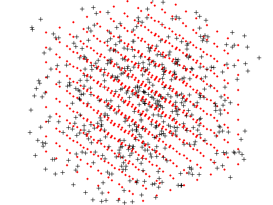
With GRIDDATAN we can interpolate X and the values v over a grid X0 to get the function values v0 over this grid.

The black points are X and the red points are the grid X0.

% Grid the data.
d  = -0.8:0.2:0.8;
[x0,y0,z0] = meshgrid(d,d,d);
X0 = [x0(:) y0(:) z0(:)];
v0 = reshape(griddatan(X,v,X0),size(x0));
% Plot results.
cla reset; hold on;
plot3(X(:,1),X(:,2),X(:,3),'k+','markerfacecolor','k');
plot3(X0(:,1),X0(:,2),X0(:,3),'r.','markerfacecolor','r');
view(3); axis equal tight off vis3d; camzoom(1.6);
rotate3d on

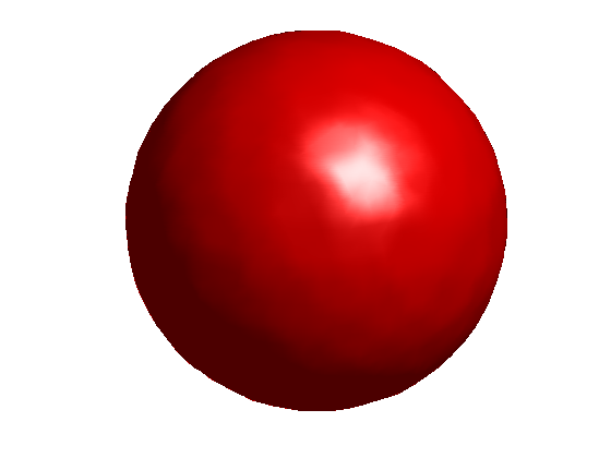
To visualize the surface at all points where the function takes on a constant value, we can use ISOSURFACE and ISONORMALS. Since the function is the squared distance from the origin, the surface at a constant value is a sphere.

c = 0.6;  % constant value
cla reset; hold on;
h = patch(isosurface(x0,y0,z0,v0,c),'FaceColor','red','EdgeColor','none');
isonormals(x0,y0,z0,v0,h);
view(3); axis equal tight off vis3d; camzoom(1.6); camlight; lighting phong
rotate3d on

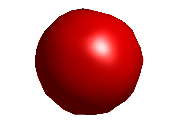
With more data points in X and a denser grid X0, the sphere is smoother but takes longer to compute.

Here is a precomputed sphere generated using 5000 data points in X and a distance between gridpoints of 0.05.

% Load saved results.
load qhulldemo
cla reset; hold on
d = -0.8:0.05:0.8;
[x0,y0,z0] = meshgrid(d,d,d);
h = patch(isosurface(x0,y0,z0,v0,0.6));
isonormals(x0,y0,z0,v0,h);
set(h,'FaceColor','red','EdgeColor','none');
view(3); axis equal tight off vis3d; camzoom(1.6)
camlight; lighting phong
rotate3d on

Copyright 1984-2007 The MathWorks, Inc.
Published with MATLAB® 7.7

MATLAB and Simulink are registered trademarks of The MathWorks, Inc. Please see www.mathworks.com/trademarks for a list of other trademarks owned by The MathWorks, Inc. Other product or brand names are trademarks or registered trademarks of their respective owners.