Finite Difference Laplacian
This demo illustrates the computation and representation of the finite difference Laplacian on an L-shaped domain.
Contents
The Domain
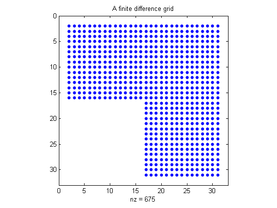
For this example, NUMGRID numbers points within an L-shaped domain. The SPY function is a very useful tool for visualizing the pattern of non-zero elements in a given matrix.
R = 'L'; % Other possible shapes include S,N,C,D,A,H,B
% Generate and display the grid.
n = 32;
G = numgrid(R,n);
spy(G)
title('A finite difference grid')
% Show a smaller version as sample.
g = numgrid(R,12)
g =

     0     0     0     0     0     0     0     0     0     0     0     0
     0     1     6    11    16    21    26    36    46    56    66     0
     0     2     7    12    17    22    27    37    47    57    67     0
     0     3     8    13    18    23    28    38    48    58    68     0
     0     4     9    14    19    24    29    39    49    59    69     0
     0     5    10    15    20    25    30    40    50    60    70     0
     0     0     0     0     0     0    31    41    51    61    71     0
     0     0     0     0     0     0    32    42    52    62    72     0
     0     0     0     0     0     0    33    43    53    63    73     0
     0     0     0     0     0     0    34    44    54    64    74     0
     0     0     0     0     0     0    35    45    55    65    75     0
     0     0     0     0     0     0     0     0     0     0     0     0
The Discrete Laplacian
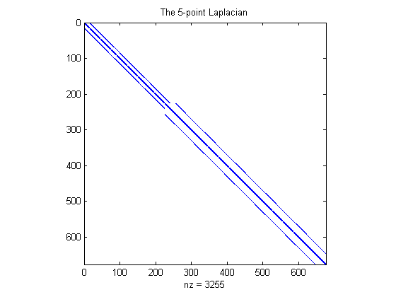
Use DELSQ to generate the discrete Laplacian. The SPY function gives a graphical feel of the population of the matrix.
D = delsq(G);
spy(D)
title('The 5-point Laplacian')
% Number of interior points
N = sum(G(:)>0)
N =

   675
The Dirichlet Boundary Value Problem
Finally, we solve the Dirichlet boundary value problem for the sparse linear system. The problem is setup as follows:
  delsq(u) = 1 in the interior,
  u = 0 on the boundary.
rhs = ones(N,1);
if (R == 'N') % For nested dissection, turn off minimum degree ordering.
    spparms('autommd',0)
    u = D\rhs;
    spparms('autommd',1)
else
    u = D\rhs; % This is used for R=='L' as in this example
end
The Solution
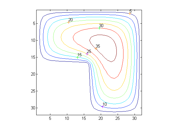
Map the solution onto the grid and show it as a contour map.
U = G;
U(G>0) = full(u(G(G>0)));
clabel(contour(U));
prism
axis square ij
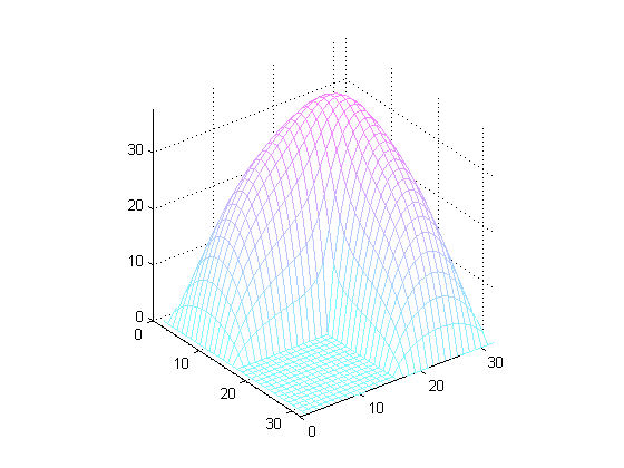
Now show the solution as a mesh plot.
colormap((cool+1)/2);
mesh(U)
axis([0 n 0 n 0 max(max(U))])
axis square ij